Object Detection in Images

Recently, there has been a lot of improvements in the Artificial Intelligence sector thanks to Deep Learning and image Processing.

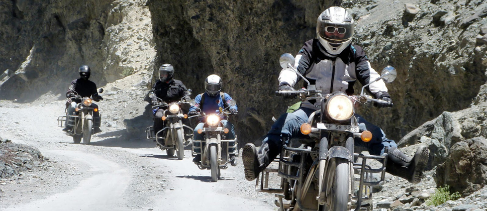
It’s now possible to recognize images or even find objects inside an image with a standard GPU. Fig.1 is an example of what could be obtained in a matter of milliseconds.

How does it work ?

In this article, the main focus will be the object detection algorithm named faster RCNN. However, in order to fully understand how it works, we will first go back in time and explain the algorithms which it was built upon. As it might take a while it will be split into two parts.

We won’t delve into all the tricky details or the underlying mathematics of theses algorithms, however a prior knowledge of the Convolutional Neural Networks theory (Convolution, Pooling, ..) would probably ease the reading.

So let’s dig a bit into the Deep Learning world !

Alexnet (2012)

We cannot talk about Deep Learning without mentioning Alexnet. Indeed, it is one of the pioneer Deep Neural Net which aim is to classify images. It has been developed by Alex Krizhevsky, Ilya Sutskever, and Geoffrey Hinton and won an Image classification Challenge (ILSVRC) in 2012 by a large margin.

At that time the other competing algorithms were not based on Deep Learning. Now, and since then, they almost all are. This net had a huge impact on the domain and most of following nets were more or less based on its architecture.

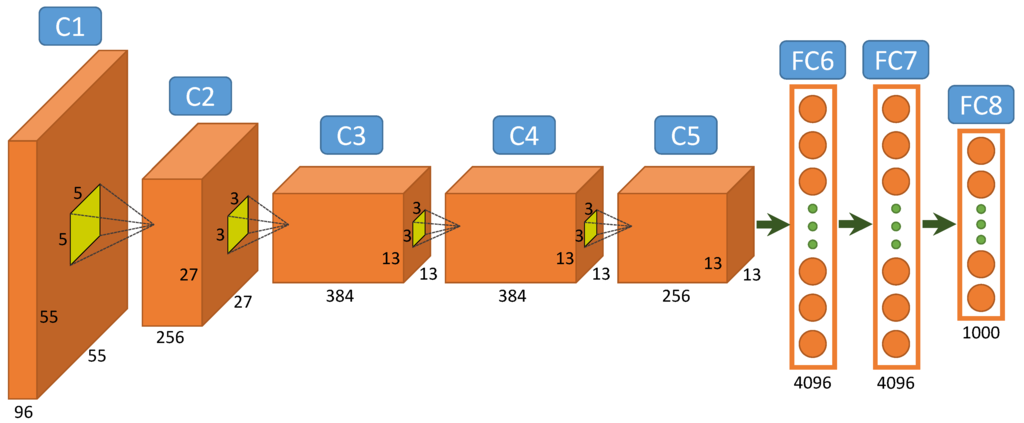
Alexnet (Fig.2) is composed of 5 convolutional layers (C1 to C5 on schema) followed by two fully connected (FC6 and FC7), and a final softmax output layer (FC8). It was initially trained to recognize 1000 different objects.

The intuition behind this net is that each convolutional layer learns a more detailed representation of the images (feature map) than the previous one. For example the first layer is able to recognize very simple forms or colors, and the last one more complex forms such as full faces for instance (see Fig.3).

The convolutional layers are representing the image in a much better way for the classification. After the convolutions, each image is represented as a vector of 4096 features (whereas they were initially vectors of 227*227*3 = 154 587 features).

The two fully connected and softmax layers are similar to a multi layer perception and could actually be replaced by other kinds of classifiers such as Random Forests or SVMs. However they are really important for the training phase of the neural net.

ZFNet (2013) and VGG (2014)

Alexnet is a very important network but the nets we are going to see aren’t actually built on it but on some of its descendents ZFNet and VGG.

ZFNet has the same global architecture as Alexnet, that is to say 5 convolutionnal layers, two fully connected layers and an output softmax one. The differences are for example better sized convolutionnal kernels.

VGG is a very deep and simple net. In the most common version, it has 16 layers (The blue pooling layers aren’t counted on the schema). However the global architecture is very similar to the Alexnet one. Actually the Alexnet convolutionnal layers are here represented by two or three following convolutionnal layers. Another difference is that each convolutionnal layers has a 3x3 kernel unlike the other nets thats have different sized kernels for each layer.

These important nets are built to classify images, that is to say to output a class when showed an image. This problem is quite well solved since today’s results beat human performances.

But let’s now focus on the main subject: Object Detection in Images. This problem is quite more difficult because the algorithm must not only find all objects into an image but also their exact locations. In other words, the algorithm should be able to detect that, on a specific area of the image (namely a ‘box’) there is a certain type of object.

RCNN (2013)

R-CNN was the first algorithm to apply deep learning to the object detection task. It beats the previous ones by more than 30% on the VOC2012 (Visual Object Classes Challenge) and was therefore a huge improvement in the fields of Object detection.

As previously mentioned, Object Detection presents two difficulties : finding objects and classifying them. That’s the point of R-CNN: dividing the hard task of object detection in two easier ones:

Objects Proposal (finding objects)
Region Classification (understanding them)

The Object Proposal task is an active research field and, in 2013, several algorithms were already performing well. We will not detail this task here but it is good to know that there are two main families of algorithms:

The ones that group super-pixels (Selective Search, CPMC, MCG, …)
The ones based on a sliding window (EdgeBoxes, …)

R-CNN is actually independent of the Object Proposal algorithm and can use any of these methods.

R-CNN takes as input the regions (or objects or boxes) proposals. Most Region Proposal algorithms output a great number of regions (around 2000 for a standard image) and R-CNN objective is to find which regions are significant and the objects they represent.

R-CNN gets parts of an image and must classify them. We saw earlier that Image Classification is a quite easy task thanks to Deep Learning nets such as Alexnet. That’s the point of R-CNN, using Deep Learning to classify each Region of Interest outputted by an Object Proposal algorithm.

R-CNN does not directly use an Alexnet on all region proposals because on top of classifying an image, the model should be able to correct the location of a region proposal if it is not right.

However, if you remember Alexnet, we saw that the fully-connected layers after the convolutions could actually be replaced by any other classifier. That’s exactly what is done in R-CNN. The convolutional part of Alexnet is used to compute the features of each region and then SVMs use these features to classify the regions. The advantage of this method is that the neural net (Alexnet) is already trained on a huge image dataset and is very powerful to feature engineer the region proposals. Before this SVM classification step, the neural net is fine-tuned to consider a new class “background”, in order to distinguish areas with or without objects.

Regions proposals, which are rectangles of different possible shapes, are transformed into squares of 227x227 pixels, the input size needed by Alexnet. They are then processed through the net and the values obtained on the last feature map are outputted. The region have then become 4096 feature vectors. These feature vector encode the images information in a much better way to process classification.

Then a one-vs-rest SVMs strategy is applied on all regions vectors. That is to say if the model is trained to recognize 100 classes, then 100 binary SVMs will be processed on each region. By keeping the best score among all binary classifier, we get the corresponding detected object class (or background actually). Even if the classifiers are all able to recognize only one class among the others, the results are good because the features extracted from Alexnet are shared among all classes.

There is then a step of regression of the bounding boxes in order to correct location of region proposals that were not good, for example if the box is not well centered on the object or not of the good ratio. This regression phase outputs correction factors to the coordinates of the bounding box. For this task, class-specific linear regressors are trained on the feature maps to predict the ground truth bounding boxes.

Eventually, there is a mechanism to keep only best regions. If a region overlaps with another one of the same class with more than a certain percentage (around 30% works quite well), only the better scored region is kept. This allows to keep a fairly reasonable number of regions.

That’s it for the R-CNN. This algorithm is powerful and works very well but it has several drawbacks:

It is very long. The region proposal takes from 0.2 to several seconds depending on the method, then the feature extraction and classification again takes several seconds. It can go up to a minute on a CPU for one image.
It is not a fluid algorithm. There are three differents steps that are almost independent and thus need a separate training.

SPP-NET

In the RCNN, each region proposal has to be inputted in a net with a fixed size (227x227 for Alexnet). That is to say every region must have the same dimension. This is a problem because obviously images and regions could be of all sizes and ratio. So, some transformations need to be performed on images to put them in the right format. Two of the most common transformations are cropping the image (only selecting a right-sized part of the image) and warping the image (changing the ratio). Both theses techniques have obvious drawbacks and might change the image in a way that will decrease the detection accuracy.

But if we look in detail at neural network layers, we can see that convolutional layers do not actually need a fixed-size input, only the fully connected layers do. Those layers are deep in the net, so there is no reason to fix the input of the net when it can be done just before the fully connected layers. That is what SPP-NET is about, they introduce a new type of layer named Spatial Pyramid pooling, placed after the convolutional layers and before the fully connected ones. This layer pools the last feature map in a way that will generate fixed length vectors for the fully connected layers. With this Spatial Pyramid pooling (see Fig.8) there is no need to warp or crop the inputted images.

But now, you may be wondering what this method has to do with our Object Detection subject. Actually, there is a direct link: R-CNN is very time-consuming because the features inputted to the SVM are independently calculated for each region proposal. For instance, if 2000 region proposals are extracted, they will be process in an Alexnet to compute their feature map one at a time. Instead, with the proposed method in SPP-Net, convolutional layers are only computed once for the entire image (and not for every region proposal). Each region proposal location is then mapped on the whole image feature map and length-fixed features are extracted from this feature map with the Spatial Pyramid pooling layer.

In this layer, the number of bins of the pooling is fixed without regarding the size of the image, whereas in normal pooling, the size of bins are fixed but not their numbers. In a Spatial Pyramid pooling layer, the size of the bins depends on the image size.

It is called a Pyramid Pooling because several pooling with different numbers of bins (so different ratios) are done in parallel (see Fig.10). For example, on the schema a pooling is done on the full image (1 bin), one is done on one quarter of the image (4 bins) and one is done on 1/16 of the image (16 bins). The results of those pooling are then simply concatenated in a vector. The idea behind the Spatial Pyramid Pooling is Spatial Pyramid Matching which is a method that was widely used in Image Recognition tasks before the emergence of Deep Learning. It is able to handle various scales, sizes and aspects ratio, which is very important in Object Detection.

Then, when the region proposal features are extracted, an SVM classification and a bounding box regression are performed on each one, the same way it is done in RCNN. However, the full process is 10 to 100 times faster at test time and 3 times faster at train time.

This algorithm still has several drawbacks:

It is still not a fluid algorithm. There are again three separate training steps.
Unlike R-CNN, the fine-tuning algorithm cannot update the convolutional layers that precedes the spatial pyramid pooling. This limitation (fixed convolutional layers) reduces the accuracy of very deep networks. For nets like Alexnet the accuracy is still very good, but for nets such as VGG16 the accuracy may drop down.

In the Next part, we will focus on fast-RCNN and on the algorithm that really produced the first image of this post : faster-RCNN.

References:

Alexnet : Alex Krizhevsky and Sutskever, Ilya and Geoffrey E. Hinton, ImageNet Classification with Deep Convolutional Neural Networks, Advances in Neural Information Processing Systems 25, 2012
ZFNet : Matthew D. Zeiler and Rob Fergus, Visualizing and Understanding Convolutional Networks, CoRR, 2013 VGGNet : Simonyan, K. and Zisserman, A., Very Deep Convolutional Networks for Large-Scale Image Recognition, CoRR, 2014
RCNN : Girshick, Ross and Donahue, Jeff and Darrell, Trevor and Malik, Jitendra, Rich feature hierarchies for accurate object detection and semantic segmentation, Computer Vision and Pattern Recognition, 2014
SPPNet : Kaiming, He and Xiangyu, Zhang and Shaoqing, Ren and Jian Sun, Spatial pyramid pooling in deep convolutional networks for visual recognition, European Conference on Computer Vision, 2014
Fast R-CNN : Ross Girshick, Fast R-CNN, International Conference on Computer Vision ({ICCV})}, 2015
Faster R-CNN : Shaoqing Ren and Kaiming He and Ross Girshick and Jian Sun, Faster R-CNN: Towards Real-Time Object Detection with Region Proposal Networks, Advances in Neural Information Processing Systems (NIPS), 2015

Other Images :