Object Detection in Images - Part 2 (en)
Object Detection in images
In the first part of this article, some very important deep Neural networks (AlexNet, VGGNet) and their use in an Object Detection task were the main focus. The algorithms presented were R-CNN and SPP-Net. Here is a reminder of their functioning (Fig.1). The main difference between the two is that with R-CNN convolutional features are computed for each region proposal which is expensive, while with SPP-Net it is done only once on the whole image.


Fig.1 R-CNN vs SPP-Net principles
However, both algorithms were multi-staged: assuming that region proposals were given, a first stage was to extract features, and a second one to classify the regions and refine their location.
Fast - RCNN
The main goal of Fast-RCNN is to improve these two algorithms by extracting the features and making an end-to-end classification with a single Algorithm. It is easier to train, faster at test time (the classification phase is almost real-time) and it is more accurate. However, this algorithm is still independent of the box proposal algorithm. So regions are still proposed apart, by another algorithm.
The principle here is similar to SPP-Net: the convolution map will only be computed once for the whole image and then each region proposal will be projected on it before going through a specific pooling layer and fully connected ones.
Like in SPP-Net, the specific pooling layer is used to produce a fixed size vector just before the first fully connected layer. This layer is called the RoI (Region of Interest) pooling layer and it is actually a special case of the SPP-Net spatial pyramid pooling layer with only one pyramid level. Keeping only one pyramid level makes the network much easier to train compared to SPP-Net (it is easier to compute its derivative during back propagation), allowing fine tuning of the convolutional layers.
The difference with SPP-Net is that following the fully connected layers, the network is divided into two outputs layers: this first one will do a classification (thanks to a simple softmax layer with N+1 outputs: N object classes + a background one) and the other one will do a regression over the four coordinates of the bounding box. The two separated training phase of the R-CNN (SVM classification and linear bounding box regression) are now inside the network itself.

Fig.2 Fast R-CNN
Deep convolutional dive
To understand the process a bit better, it’s interesting to plot visually what is going on with the RoI pooling layer during a forward pass. However, to get things clear let’s first focus on the convolutional layers functioning:
A convolutional layer is composed of weights gathered as a kernel (or a filter) and it produces a convolutional map (or feature map, activation map) by convolving this filter across the dimensions of an input (an image or the output of another convolutional layer) as you can see in the figure below.

Fig.3 A kernel (in red) is convolved across an image (in yellow) to produce a convolutional map (in blue)
For example, if a convolutional layer has a kernel of size 3*3, each entry of the convolutional map will be calculated as the dot product of 9 pixels values with the weights of the kernel. In a classic RGB image, a pixel is defined by three values. Each entry would actually be the sum of 27 weighted values (9 pixels * 3 colors values). Depending on the size of the kernels and on the way it is convolved across the input, it is possible to vary the size of the convolution produced map.


The group of pixels used in the input image to produce one entry on a convolutional map is called its receptive field. So an entry actually contains a bit of information from all the pixels composing its receptive field. For the first convolutional layer the receptive field is actually as large as the kernel. However, for deeper layers an entry might have a receptive field that takes half the pixels of the image for example.


When inputted in a neural network, an image will successively pass through several convolutional layers. As we saw, convolutional layers actually gather the information contained by several pixels together. The convolutional neural networks principle is that each layer will project its input on a feature map of decreasing size. This way, the pixels information will actually be compressed more and more by each layer.
In neural networks compression, it may be seen as generalization: as the network gradually compresses the information, it is able to find pixels patterns that are similar in different images. If a specific pattern is present in several images of the same object, it might be an indicator that this image represents the same object as well.
The patterns found by the successive layers are increasingly complex because the receptive fields of entries on the feature map gets bigger for each layer. For example, the first layers might find simple color or shape patterns while deeper layers might find complex ones like a wheel or a helmet. The neural network will then use these patterns presence information to make the classification.
Compression allows generalization, however, in the end the neural networks still needs enough information in its fully connected layers to be able to take meaningful decisions. That’s why a convolutional layer does not output only one convolutional map, but several. Thus, a convolutional layer is actually composed of several kernels. Each kernel will search for different patterns in the image.

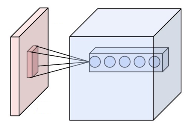
Fig.6 A convolutional output volume is composed of several convolutional maps. Here are 5 convolutional maps produced by five different kernels. Corresponding entries on all the 5 convolutional maps (like the five entries in the rectangle) encode the information of the same receptive fields but in different ways, allowing more information to pass through.
In a typical network, the successive convolutional layer outputs an increasing number of convolutional map to “counter” the compression and keep enough information (For instance, a convolutional maps of size 32*64 would not be enough to encode the information contained in a 900*450 image, but some hundred of these maps might).
During the training, the weights in the kernels are modified and learnt in order to detect specific patterns. Those patterns are determined by the training dataset and the problem to solve and they become increasingly complex the deeper we go.
However a complex pattern can be seen as a combination of more simple ones. Actually this is how we think human babies are representing and learning things (composing what they already know to understand new things). This explains the layered layout of neural networks: the first convolutional layers find simple patterns and by aggregating and combining those simple patterns, the following layers can find more complex ones.
This is one of the reason of Deep Learning generalization success: the first layers are able to learn general rules that are not specific tasks and thus can be used for other things. This explains the effectiveness of fine tuning and transfer learning (Using a neural network trained on a specific task and modifying it just a little bit to accomplish a different task). When a network is fine tuned, we base on its trained general knowledge and a little bit of task-specific understanding is simply added.
Now it is enough about the theory, let’s see how things are going when our image is processed through our network. We will focus on one region proposal (in red).

Let’s first take a look at the output of the last convolutional layers. The feature map is composed of 256 convolutional maps of size 32*64 that are represented here as a 16*16 matrix, each box being a convolutional map.

Fig.7 Last layer convolutional map
As it’s not really enlightening to show all these convolutional maps at once, let’s focus on only one, the one highlighted on the feature map

On these features maps a red pixel indicates a high value and a blue pixel a small value, following this colormap :

A high value on the feature map is what we call an activation. An activation says that a useful pattern for the classification is present there. As a reminder, this pattern is “described” by the successive kernels of the convolutional layers.
So, this activation map describes the presence of a particular pattern in the whole image, but in Object Detection we are only interested in the sub-image representing our region proposal. We can actually project this region proposal on the convolution map and then only focus on the projected part.

In order to get fixed size information for the following layers of the net, the RoI pooling layer will cut the region proposal into 6*6 smaller regions. Like in SPP-Net, these regions aren’t fixed in size, they actually depends on the region proposal size.

Something like this shoulb be obtained:

Fig.8 RoI Pooling Layer
Then for each region, only one value is kept thanks to a max pooling. This gives us a 6*6 matrix (shown here as an image)

This 6*6 matrix is then flattened into a vector of size 36.

This vector represents the information for one of the 256 activation maps. The corresponding entries on all the activation maps contain information about the same region of the input image but compressed in different ways, so they are all useful. That is why this step is done for all the 256 activation maps.
We then get 256 vectors of size 36 that are simply concatenated into a big vector (256*36 = 9216 features). This vector contains all the information the convolutional layers find relevant for the classification. The rest of the network will then use this vector to take its decision.
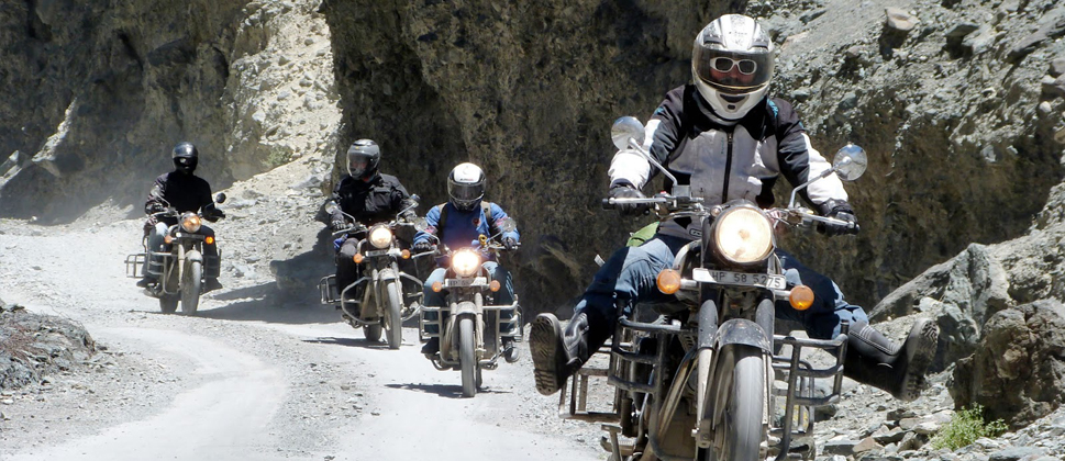
The fast-RCNN network will finally output the class of this region proposal (a motorbike) and possibly an offset to the bounding box coordinates.
Faster - RCNN
With Fast-RCNN, real-time Object Detection is possible if the region proposals are already pre-computed. However this task may take from around 0.2 seconds to one or two seconds for one image depending on the method.
This is the main point of Faster-RCNN: making the region proposals algorithm as a part of the neural network. It merges Fast-RCNN with a Region Proposal Network producing better object detection results and in real-time (hence the name :)) for the first time. Moreover, the results are not dependent on the accuracy of an external region proposals algorithm anymore.
Like Fast RCNN, a faster RCNN network may be built upon different already existing networks. Some modifications have to be made, but only after the convolutions layers. Two branches will follow these layers:
- A first one, the RPN (Region Proposal Network) that will produce the region proposals based on the last feature map.
- A second one, the fast RCNN network that will classify the RPN proposals

Fig.9 Faster-RCNN
The RPN network is as a full convolutional net that will slide on the feature map and that will tell for each position if there is an object or not (with probability and potentially bounds offset), without regards to the class of the object.
In order to have a system that is robust to translation and scale, the RPN uses an algorithm based on anchors. For each position of the sliding window on the feature map, 9 anchors are placed. The anchors are all centered on the sliding window, only their scale and ratio change (There are three scales and three ratios (1:1 , 2:1 and 1:2), making the 9 anchors.

Fig.10 Anchors in the RPN
Each anchor is processed through the convolutional layers of the RPN and the networks output the probability that this anchor represents an object and potentially an offset to correct the anchor dimensions. For example, if the object is very long, a 2:1 ratio might not be enough to cover it, so the RPN will output offset to change the anchor ratio.
If the feature map on which the sliding window is applied has a height H and a width W (For our motorbike example, H = 32, W = 64), there are H*W*9 anchors produced (18432 anchors) and tested (processed by the convolutional layers of the RPN). On a classic object image, usually around few thousands are considered as representing objects (and the others are considered as background) and only the top N are kept (Based on classification probability). It was tested experimentally that keeping around 300 proposals gives good results. The second part of the net is a classic Fast-RCNN. It will process the 300 proposals provided by the RPN to extract a fixed length vector of the feature map and classify the object.
A faster RCNN is a complex network and the training is not an easy task. There are several tricks and methods used for the training that won’t be detailed here except for one as an example: In order to train the RPN, ground truth anchors must be generated to be compared with the anchors produced by the RPN, so that the network learns if the anchors he is producing are good or not.
For our bike image that would mean to generate 18432 ground truth anchors which is expansive. That’s why only a random subsample of around 250 anchors are generated for each image. However, the number of negatives anchors is way above the number of positives ones in a normal image. So the subsampling is actually built to have about half positive and half negative anchors. Without this step the RPN would be biased toward negatives anchors as they are way more represented. This is an example of a method that is needed for the training but there are others and they need to be done on the full training dataset.
Two methods are discussed in the paper to train the full faster-RCNN network. The first one was made because of a short deadline and no theoretical assumptions that the other methods would actually work. The second method actually works even if it is based on an approximation and it is faster and easier to train with similar results.
- Alternating training: In this method, the RPN is trained first, followed by the Fast-RCNN that is trained with the proposals. Then the Fast-RCNN is fine tuned by the RPN and as a last step the RPN is fine tuned by the Fast-RCNN. This is not a simple pipeline and you need to run several trainings which is not the best. This training method is actually a way to fake a single net but the RPN and the Fast-RCNN are actually separated.
- Approximate joint training: In this method, there is really only one single net. For the optimization in the shared layer, both the RPN and fast-RCNN errors are combined. This method is called approximate because during the learning, a calculation simplification is performed (a part of the derivative is ignored during the backpropagation).
We mainly discussed Fast-RCNN and Faster R-CNN as based on AlexNet or VGG but they are actually now based on more recent Deep Learning Network which makes their accuracy better and better. For example in the recent Tensorflow Object Detection API, you can find a Faster RCNN based on ResNet and another one based on Inception ResNet v2. Those two algorithms are recent deep neural networks performing very well in Image Classification tasks.
Object Detection algorithms continually improve with the Image Classification deep neural networks they are based on. However, object detection is still an active search field and new algorithms are also being created regularly. Here are some of the best performing new methods :Yolo, R-FCN, SDD.
References:
- Fast R-CNN : Girshick, R. (2015). Fast r-cnn. In Proceedings of the IEEE international conference on computer vision(pp. 1440-1448).
- Faster R-CNN : Ren, S., He, K., Girshick, R., & Sun, J. (2015). Faster R-CNN: Towards real-time object detection with region proposal networks. In Advances in neural information processing systems (pp. 91-99).
- ResNet : He, K., Zhang, X., Ren, S., & Sun, J. (2016). Deep residual learning for image recognition. In Proceedings of the IEEE conference on computer vision and pattern recognition (pp. 770-778).
- Inception : Szegedy, C., Liu, W., Jia, Y., Sermanet, P., Reed, S., Anguelov, D., … & Rabinovich, A. (2015). Going deeper with convolutions. In Proceedings of the IEEE conference on computer vision and pattern recognition (pp. 1-9).
- SSD: Liu, W., Anguelov, D., Erhan, D., Szegedy, C., Reed, S., Fu, C. Y., & Berg, A. C. (2016, October). Ssd: Single shot multibox detector. In European conference on computer vision (pp. 21-37). Springer, Cham.
- Yolo: Redmon, J., Divvala, S., Girshick, R., & Farhadi, A. (2016). You only look once: Unified, real-time object detection. In Proceedings of the IEEE Conference on Computer Vision and Pattern Recognition (pp. 779-788).
-
R-FCN : Dai, J., Li, Y., He, K., & Sun, J. (2016). R-fcn: Object detection via region-based fully convolutional networks. In Advances in neural information processing systems (pp. 379-387).
- Tensorflow Object Detection API : https://github.com/tensorflow/models/tree/master/research/object_detection
Other Images :
- https://github.com/vdumoulin/conv_arithmetic
- https://medium.com/@nikasa1889/a-guide-to-receptive-field-arithmetic-for-convolutional-neural-networks-e0f514068807
- http://himalayanrider.com/wp-content/uploads/2013/11/motorbike-tour1.jpg
- https://upload.wikimedia.org/wikipedia/commons/6/68/Conv_layer.png